Introducing the variogram
It is nearly impossible to talk about the analysis of Precision Agriculture data without mentioning the variogram. Be aware that some people will refer to the term semi-variogram instead. There is some kind of confusion between these two terms (Bachmaier et Backes, 2008).
Some authors talk about semi-variogram because of the factor 2 at the denominator of the equation in the next section (semi as half the variogram). However, this factor 2 has been put into place because the variance is calculated twice for each pair of points (for the pair (i,j) and for the pair (j,i) while the variance is similar). For simplification purposes, both terms will be used to define the same approach. This widely used tool has been created to describe the spatial correlations of punctual spatial observations. The objective is to evaluate if a given variable follows a specific pattern in space.
For instance, a farmer might want to know if the soil characteristics inside his fields (ex: organic matter or phosphorus content) exhibit a strong spatial structure or not before considering the possibility of a variable rate fertilization. Indeed, if a field is well spatially-structure, site-specific management is much more profitable. In that case, soil samples would have to be collected within the field at specific spatial positions and a semi-variogram analysis could be performed.
The semi-variogram is the first step towards the mapping of a variable over a whole field or more generally a spatial entity. This mapping process is known as interpolation. Indeed, for practical and visual purposes, it is much more interesting to dispose of a complete mapping of the variable of interest instead of only punctual spatial observations. One important statement to make is that the semi-variogram is flawed when the number of punctual observations is not large enough. From a general perspective, a rule of thumb of at least 30 or 40 observations should be kept in mind.
Computation of the semi-variance
The semi-variogram can be computed via the following equation :
\gamma(h)=\dfrac{1}{2N(h)}\sum_{i,j\in{N(h)}}(z_i-z_j)^{2}Where N(h) stands for the number of pair observations (i,j) separated by a spatial distance h. The terms z_i and z_j are the attribute values of observations i et j respectively.

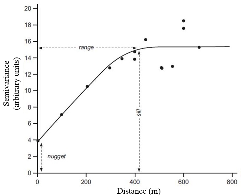
Figure 1. Theoretical exponential semi-variogram model with corresponding parameters
This function calculates the attribute difference between neighbouring observations separated by a lag h to evaluate if these observations display the same information. As it was stated in a previous post, agronomic observations generally exhibit some spatial correlations. Regarding the semi-variogram, it means that as the distance between observations increases, the semi-variance is likely to increase because near observations share more characteristics than distant ones (Fig. 1). In Figure 1, the black points sum up the spatial structure of the entire dataset. In fact, the semi-variogram is computed for all pairs of observations but the plot would be unreadable if all the semi-variances were reported. One of the strongest assumption of the variogram is that of second-order stationarity, the fact that the variogram is bounded and reaches a plateau. To have more information about the fundamental assumptions of the variogram, check out this post ! From the semi-variance functions, several parameters have been derived to describe the field spatial structure
Variogram parameters
The nugget effect, often referred to as C_0, represents the small-scale spatial variations within the fields. This is an indicator of how noisy the spatial structure is. For instance, inside the fields, there exists some plant to plant variability since plants are living elements. Not all neighbouring plants can be exactly similar. When the minimal distance between neighbouring observations is too large, the nugget might be found higher than it should be. This is because the semi-variogram is not able to embrace all the spatial structure in the field, and especially at small-scales. It must be said that small-scale variations can also be due to measurement errors, more especially from a man-made or sensor measurement. The partial sill, C_1, represents the magnitude of variation of the variable of interest. Intuitively, the higher the partial sill compared to the nugget, the stronger the spatial structure. The sill is the variance of the dataset and can be computed as the sum of the partial sill and nugget. The sill corresponds to the value when the semi-variances reaches a plateau and stabilizes. Last but not least, the range, a, is the distance beyond which observations are no longer spatially correlated. It is considered that in average, above a specific spatial distance and whatever the pair of points examined, observations are too dissimilar and do not share any relationship.
To better characterize the above spatial structure, there is a need to fit known functions to the semi-variogram. These functions will help give an objective description of the spatial correlation of the data under study and retrieve the aforementioned parameters C_0, C_1 and a.
Fitting a variogram model to the data
Before describing well-known semi-variogram models, it must be understood that all these models are theoretical which means that there is a strong probability that these models will not fit exactly to the data under study.

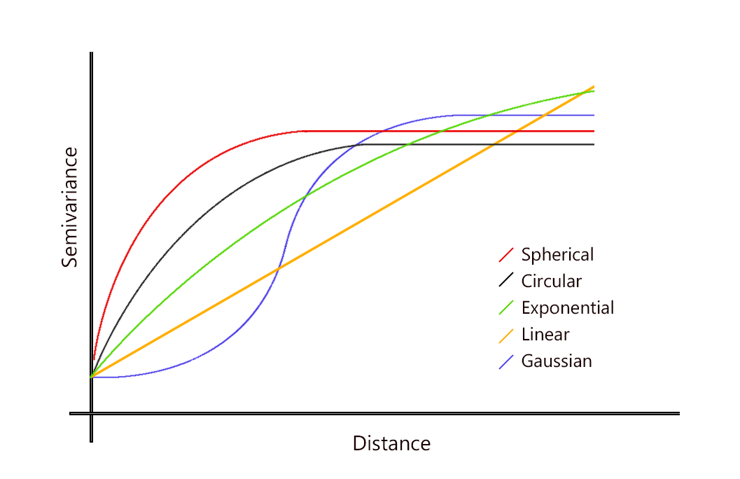
Figure 2. Most common theoretical variogram models
Figure 2 shows the most commonly-used semi-variogram models. In agronomic studies, theoretical exponential and spherical models are often employed to fit to edaphic (soil nutrient content) and plant parameters (vigour, NDVI….). On this two models, the nugget and partial sill parameters are relatively easy to find. As it was previously stated, the range is the distance beyond which observations are no longer correlated, that is to say when the semi-variance reaches a plateau. From a theoretical point of view, the semi-variance actually never reaches the plateau but tend to it. Does this mean that the range cannot be defined ? No, obviously. Instead of the theoretical range, a pratical range has been put into place to overcome the problem.
For instance, for the exponential model, the range is defined as the distance at which the semi-variance reaches 95% of the sill.
Linear models tend to increase indefinitely. These models are often the sign of a trend in the data.
For example, in the case of an elevation gradient (on a slope), the elevation increases in the direction of the gradient which means that there is a trend with regard to the spatial coordinates. This trend would need to be removed first in order to evaluate the real spatial structure of the elevation variable.
Last discussed models refers to a pure nugget effect. In that case, there is absolutely no spatial structure; the process is totally random. There is either too much noise in the data or the variable effectively does not exhibit eany spatial correlation.
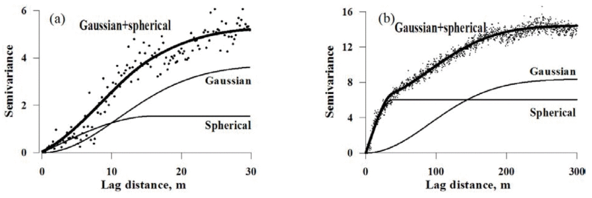
So far, all the spatial structures that were presented are relatively simple. Once again, these models are theoretical and real semi-variance functions generally deviates from these models. In some cases, it might be possible to have nested models to fit to the data (Fig. 3). In fact, there might be multiple spatial structures whithin the field at different spatial scales. Here, it would be interested to fit the two theoretical semi-variogram models to embrace the entire spatial structure within the dataset.

Figure 3. Modèle gigogne de semi-variogramme avec deux structures spatiales
Isotropic and anisotropic semi variograms
An isotropic phenomenom is a process that is not directionnaly dependent. In spatial studies, this process is considered to evolve similarly in all the directions in space. On the contrary, anistropy refers to a process that varies differently according to the direction of interest.
Assume for instance that you want to perform a species diversity analysis along a hillslope. There is a strong probability that the differences in species diversity are intensified at varying elevations than are the same elevation. Results would be much more interesting if the analysis is performed in the direction of the slope. Here, the use of a directional variogram would be recommended.
Sometimes, anisotropic models enable to derive conclusions that would not have been found with a isotropic modelling.
Last remarks and discussion
The semi-variogram is a very valuable tool to analyse the spatial structure of agronomic and environmental spatial datasets. However, some issues need to be discussed to avoid misinterpretations or an inappropriate usage. First of all, it must be kept in mind that the choice of the semi-variogram model to fit to the data will influence the values of the variogram parameters (range, nugget and sill).
For instance, according to the same data, an exponential semi-variogram model will lead to a smaller range than a spherical one.
It is possible to calculate some measures of goodness of fit to help choose the best variogram models but when multiple models might be used, care must be paid. Also, depending on the way the semi-variance is averaged over specific lags (for example, an average every 5, 20 or 50m), the semi-variogram might look different. For all these reasons, I would recommend to always work on variograms with a manual supervision. According to me, the complete automation of semi-variogram analysis might lead to misleading conclusions.
The semi-variogram is relatively easy to compute (several R packages are available, check out this post). Once again, I would like to call your attention to the fact that the computation of a semi-variogram requires a minimum number of observations. When the number of observations is too small (<30), the semi-variance function is not reliable. Sometimes, in the literature, it happens that soil spatial structure studies are performed with ten to twenty samples (and sometimes less). This is understandable because soil sampling is relatively costly and cumbersome. However, a semi-variogram computation with 10 observations does not make any sense.
In the introduction, the semi-variogram computation was presented as a first step towards the interpolation of the variable under study. The semi-variogram might also be used to determine an estimate of the optimal sampling distance between observations.
For instance, a NDVI image could be used to evaluate the sampling distance to use during a soil sampling campaign.
A rule of thumb is to consider half the range of the semi-variogram as a good indicator of the sampling distance between observations.
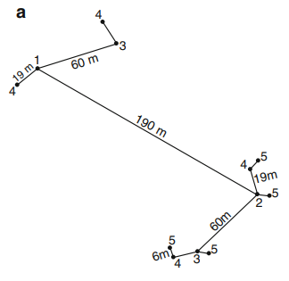
As you have certainly understood, the semi-variance is calculated for multiple lags between observations. To obtain the best possible variogram, it would be necessary to have lots of different spatial distances between the observations. One possible sampling scheme would be not to locate regularly the samples to better characterize the whole spatial structure(s) whithin the field (Fig. 4).

Figure 4. Exemple d’échantillonnage spatial non régulier
So far, the semi-variogram analysis has only be presented to evaluate the spatial correlation of a given variable. However, keep in mind that it is possible to study the spatial structure of a first variable compared to a second one. In that case, the semi-variogram turns into a cross-variogram.
For instance, this kind of analysis is interesting when one variable is easy and cheap (X) to acquire while the other is much more cumbersome and costly to obtain (Y). A cross-variogram would be valuable to evaluate the cross-correlation between the two variables (the spatial structure of X given that of Y ). It will then be possible to interpolate Y (from which few observations are available) by making use of the cross-correlation previously determined.
Support Aspexit’s blog posts on TIPEEE
A small donation to continue to offer quality content and to always share and popularize knowledge =) ?


1 thought on “Variogram and spatial autocorrelation”