The simulation of fields with varying spatial structures is an interesting strategy when it comes to testing or evaluating a specific processing method. The main advantage of simulations is that one is able to control the data distribution within the field so that the context under which the processing method is applied is well-known.
For instance, one might want to confront an outlier detection method to noisy datasets.
The package gstat provides powerful and efficient functions to create spatially-structured datasets. This package can effectively be used to simulate these Gaussian random fields (the term commonly used by spatial analysts) via the sequential simulation algorithm (Bivand et al., 2013) 1. This approach requires to define a model for the semi-variogram that will be used to create the random fields. The sequential simulation algorithm uses the variogram model and previously simulated values to compute the conditional distribution of future observations. A new observation is selected from that conditional distribution and added to the dataset. These steps are repeated until all observations are given a value (Bivand et al., 2013). Note that another interesting post tackles the simulation of these gaussian random fields in R.
## Load the package gstat
library(gstat)
## Create a square field of side 100. The field can be seen as a grid of regularly spaced pixels
Field = expand.grid(1:100, 1:100)
## Set the name of the spatial coordinates within the field
names(Field)=c('x','y')

## Define the yield spatial structure inside the field
   ## Set the parameters of the semi-variogram
      Psill=15  ## Partial sill = Magnitude of variation
      Range=30  ## Maximal distance of autocorrelation
      Nugget=3  ## Small-scale variations
   ## Set the semi-variogram model
      Beta=7   ## mean yield (tons/ha) in the field
      RDT_modelling=gstat(formula=z~1, ## We assume that there is a constant trend in the data
                           locations=~x+y,
                           dummy=T,    ## Logical value to set to True for unconditional simulation
                           beta=Beta,  ## Necessity to set the average value over the field
                           model=vgm(psill=Psill,
                                     range=Range ,
                                     nugget=Nugget,
                                     model='Sph'), ## Spherical semi-variogram model
                           nmax=40) ## number of nearest observations used for each new prediction

## Simulate the yield spatial structure within the field
RDT_gaussian_field=predict(RDT_modelling, newdata=Field, nsim=1) ## nsim : Nombre de simulations
The variable RDT_gaussian_field is a data frame that contains, for each observation inside the field (each pixel), the spatial coordinates and the associated yield value. In order to display the simulated spatial structure, the package ggplot2 can be used as follows:
## Load the package ggplot2
library(ggplot2)

## Plot the field
ggplot()+  ## Initialize the ggplot layer
geom_point(data=RDT_gaussian_field,aes(x=x,y=y,col=sim1))+ ## plot the observations as points with a colored yield gradient
scale_colour_gradient(low="red",high="green")   ## Set the colors of the gradient
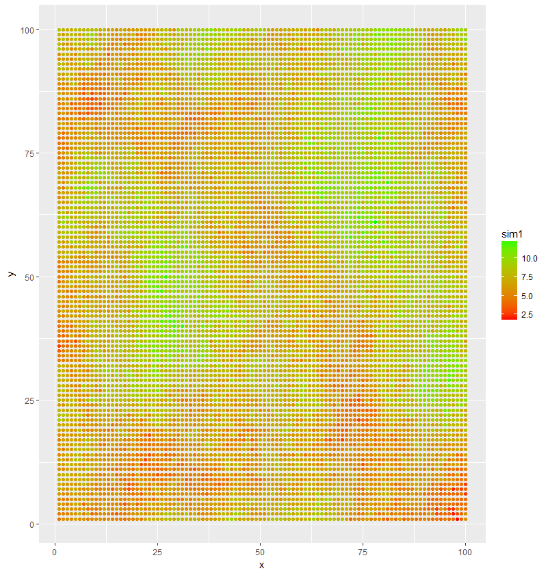
A single run of the simulation led to the following field (Fig. 1):

Figure 1. Simulated field with a relatively good yield spatial structure
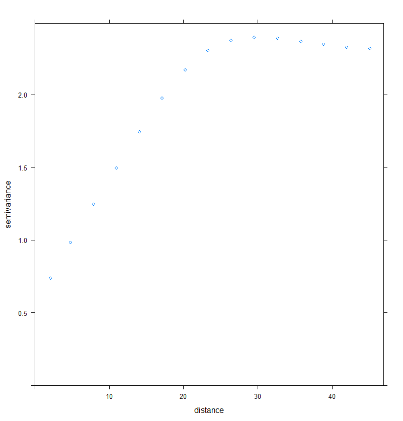
It has to be understood that the simulation intends to recreate the spatial structure with the semi-variogram parameters that were set. However, it may happen that the simulated spatial structure differs from the desired one. It is not really the case here. Figure 2 shows the spatial structure of the previously simulated dataset. The estimated sill (partial sill + nugget) seems to be slightly higher than the setting. Nonetheless, from a general perspective, the spatial structure is well-respected.

Figure 2. Spatial structure of the simulated dataset
A small donation to continue to offer quality content and to always share and popularize knowledge =) ?
- Bivand, R.S., Pebesma, E.J., & Gomez-Rubio, V. (2013) Applied Spatial Data Analysis with R. New York, NY: Springer

