Generally speaking, when we want to evaluate the robustness and/or generality of an algorithm, we need to test it on a large number of data, with quite varied characteristics, to ensure that the algorithm will give conclusive results in the vast majority of cases. If we had the means to have real data or field data in large enough quantities, we could afford to test the algorithm on that data. Unfortunately, for obvious reasons of cost, time or difficulty of acquisition, we have little access to significant sources of real data. To overcome this problem, one can work with theoretical data by doing simulation, making sure that the simulated data resemble the real data as much as possible (otherwise, there would be little interest in simulation…).
In Precision Agriculture, spatial data exhibit correlation structures, especially spatial (but not only), which must therefore be recreated when doing simulation. In a previous post, we saw how to simulate a spatial agronomic variable on a plot with a given spatial structure. In this post, we will see how to simulate two spatial agronomic variables on the same plot, these two variables being correlated with each other. This post was written based on the article by Baptiste Oger [“Combining target sampling with within field route-optimization to optimize on field yield estimation in viticulture”] submitted in the journal “Precision Agriculture” in 2020. The article focuses on the development of a new sampling optimization method to better estimate the yield of a vineyard plot (interested readers can have a look at it – it talks about constrained optimization- but it is not directly the subject of this post). In this work, the authors hypothesize that, under certain soil-climate conditions, crop yield is correlated to a vegetation indicator (NDVI) of the crop. By using this vegetation information as auxiliary information (more readily available than yield) to select sampling points of interest, it would then be possible to facilitate and improve yield estimation in the plot. To test the relevance of their sampling method, one of the prerequisites of this paper was therefore to be able to generate simulated yield and NDVI data, more or less correlated with each other …
Presentation of the method for generating cross-correlated spatial data
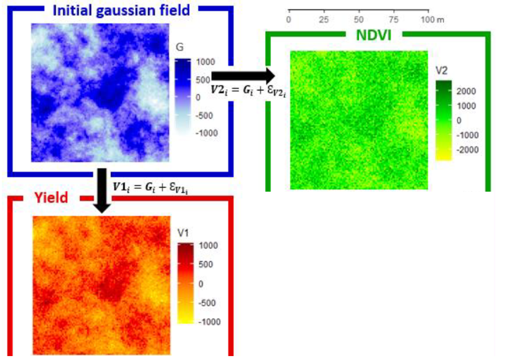
The general idea behind the method is relatively simple. The first step is to create a spatial variable G on a given plot (in the same way as presented in a previous post) except that here we create this variable without any nugget effect. The data for this variable are therefore not noisy at all, the whole variability is spatially structured (if one were to represent the spatial structure using a variogram, the variogram would pass through the origin (0.0) of the graph). From this spatialized variable G, which is used as a reference, two agronomic variables – V1 and V2 – will be created. Using the case study from Baptiste’s paper, V1 can be equated to the yield layer and V2 to the NDVI layer. A noise layer (E_{V1}) will be added on G to build V1, and a different noise layer (E_{V2}) will be added on G to build V2. The noise added to G is random, it has no spatial structure. It’s a pure nugget effect, so to speak. Depending on the characteristics of the initial G variable, and the noise that will be added, we can play on three criteria:
- The spatial auto-correlation distance of G, V1 and V2 (this is the range of the variogram),
- The proportion of noise in the data of V1 (one cannot control at the same time that of V1 and V2 so one fixes that of V1 first, and one can work on that of V2 according to what one has done for V1). This proportion of noise is also called the small-scale variance.
- The degree of correlation between the variables V1 and V2 can be seen in the table below.
We are now going to represent some equations to go into a little bit more detail about this method. I promise, nothing too complicated! Figure 1 below will allow you to better understand the method before starting the theoretical part.

Figure 1. Generation of two correlated spatialized variables
Theory of the method
Let’s start by defining some notations:
- G is a regionalized variable with no nugget effect.
- E_{V1} is the noise variable that will be added to G to construct V1. E_{V1} is a variable with a Gaussian distribution centered on 0 with a variance \sigma^2_{EV1}.
- E_{V2} is the noise variable that will be added to G to construct V2. E_{V2} is a variable with a Gaussian distribution centered on 0 with a variance \sigma^2_{EV2}.
- We will construct the variables G, E_{V1}, E_{V2}, V1 and V2 on a 100m x 100m grid, with pixels of 1 meter side. So there will be 10000 data for each variable. We add the notation for the index “i” to characterize the “ith” data. We can thus define G_i, E_{V1i}, E_{V2i}, V1_i or V2_i.
To build G, we saw how to do it with R in a previous post. We can indeed simulate a Gaussian field by filling in the variographic parameters we want (nugget, span, total variance). Here, the nugget effect is set to 0 because I remind you that we want to generate a regionalized variable without any nugget effect. The scope of the variogram that will be defined for G will indirectly be the same as for V1 and V2 (adding the E_{V1} and E_{V2} noises will not affect the scope of the variograms for V1 and V2).
Following what has been defined above, we simply define the variables V1 and V2 at each point “i” as follows:
V1_i=G_{i}+E_{V1i} with E_{V1i} \sim N(0,\sigma^2_{EV1})
V1_i=G_{i}+E_{V2i} with E_{V2i}\sim N(0,\sigma^2_{EV2})
Since the noise variables E_{V1} and E_{V2} follow a Gaussian distribution centered on 0, the only parameters that can be played to influence the criteria the proportion of noise in the data of V1 or the degree of correlation between V1 and V2, these are the variances \sigma^2_{EV1} and \sigma^2_{EV2} of the variables E_{V1} and E_{V2}.
Let’s first work on the proportion of noise for V1.
Let C_{1} be the proportion of noise (small-scale variance) for V1.
C_{1} = \frac{Nugget Effet of V1}{ Total variance of V1}
Since the reference variable G is a variable without a nugget effect, the nugget effect of V1 is simply the variance of E_{V1}. The total variance of V1 is the same as the variance of G since only noise has been added to G.
C_{1}= \frac{\sigma^2_{EV1}}{\sigma^2_{G}+\sigma^2_{EV1}}
By isolating \sigma^2_{EV1} on the left of the equation,
\sigma^2_{EV1} = \frac{C_{1} \times \sigma^2_{G}}{1-C_{1}}
We can thus play on the proportion of noise in V1 by varying the value of C_{1}, for a fixed total variance of G.
Let us then work on the correlation between V1 and V2
Let’s look at the covariance between the variables V1 and V2 before looking at the degree of correlation between V1 and V2. The covariance is simply written :
Cov(V1,V2)=Cov(G+E_{V1},G+E_{V2})
Decomposing the previous equation with the covariance formula, we get:
Cov(V1,V2)=Cov(G,G)+Cov(G,E_{V1})+Cov(G,E_{V2})+Cov(E_{V1},E_{V2})
Variables G, EV1, and EV2 are all random variables. Each one is also independent of the other. The theory tells us that the covariance of two independent random variables is zero. The previous equation can therefore be simplified:
Cov(V1,V2)=Cov(G,G)=Var(G)=\sigma^2_{G}
We have just decomposed the formula of the covariance – Cov(V1,V2) – but what interests us is to be able to choose the correlation between the variables V1 and V2 – Cor(V1,V2). The covariances and correlations between V1 and V2 are related by the Pearson formula :
Cor(V1,V2)=\frac{Cov(V1,V2)}{\sqrt{Var(V1)}}
By replacing the terms in the equation,
Cor(V1,V2)=\frac{\sigma^2_{G}}{\sqrt{\sigma^2_{G}+\sigma^2_{EV1}} \sqrt{\sigma^2_{G}+\sigma^2_{EV2}}}
Finally, by rearranging the equation, we are able to define how to adjust the noise of the variable V2 according to the degree of correlation between V1 and V2:
\sigma^2_{EV2}=(\frac{\sigma^2_{G}}{\sqrt{\sigma^2_{G}+\sigma^2_{EV1}} \times Cor(V1,V2)})^2-\sigma^2_{G}
There you go! What the previous equations show us is that we know how to set the noise variables E_{V1} and E_{V2} to have the proportion of noise in space for V1, and the degree of correlation between V1 and V2 desired. For example, if I set a noise ratio of 0.3 for V1, and I want the correlation between V1 and V2 to be 0.7; I can calculate \sigma^2_{EV1} and \sigma^2_{EV2} accordingly and have the expected variables V1 and V2.
Some little extras
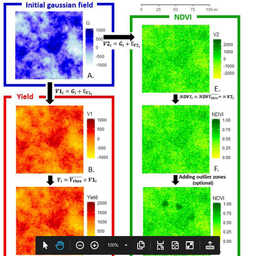
To go a little further in data simulation, two options are considered in Baptiste Oger’s article. Don’t worry, it’s simpler than what was presented above. These options are presented in Figure 2.
The first is to rescale the data values of the variables V1 and V2. Typically, a negative yield value does not make much sense. Similarly, NDVI vegetation values are more likely to be in the range of 0 to 1. For example, to more accurately represent the yield (Y) and NDVI variables, the V1 and V2 data can be linearly transformed by setting the mean value of the expected yield (Y) and NDVI variables and their level of variance.
Y_{i}= \bar{Y} + V1_{i}
NDVI_{i}= \bar{NDVI} + V2_{i} \alpha
With \bar{Y} and \bar{NDVI} being the mean Yield and NDVI being expected.
These transformations in no way affect the parameterization we saw above, namely the range of the variogram of G, V1 and V2; the noise ratio of V1, or the correlation between V1 and V2.
The second option is to model somewhat specific phenomena in the plot – localized disease areas, group of missing plants at certain places in the plot – to have a better representation of reality. Note that zones will be added to the variable V2 (NDVI) to make the correlation structures between V1 and V2 more complex. These phenomena, which are quite localized in the plots, are rather difficult to model by a simple addition of random noise as we did with E_{V1} and E_{V2}. It could happen, of course, but it would require that, in a random way, several noises on nearby data would have to be very strong or very weak (which will not happen very often…). Baptiste proposes instead to select a small number of neighbouring data to constitute a zone, and to assign the same value to all the data in this zone, this value being either abnormally high or abnormally low in relation to the expected NDVI average. A fairly simple filter can be used to smooth the data around the zone so that there are no abrupt changes in values between the inside and outside of the zone (in reality, there are more data gradients in the plots than very abrupt changes). This process can be repeated for as many areas as you want to show on the plot.
With this post and one of the previous ones, you are now able to simulate not only one auto-correlated variable in space, but also two spatially correlated variables!

Figure 2. Generation of two spatially correlated variables – improving the variable to match reality
Support Aspexit’s blog posts on TIPEEE
A small donation to continue to offer quality content and to always share and popularize knowledge =) ?

